Working with units in MEEP is easy. The quantities which we are measure like transmitted/reflected power, etc are all unitless. Before diving into the methods, lets look into key concepts.

Scalar Invariance:

Scalar invariant laws do not change on multiplying or dividing  by a common factor. For example consider a homogenous function f(x). If we are scaling 'x' to 'sx' ,

$\begin{eqnarray*}f(sx)= (constant) \times f(x)\end{eqnarray*}$

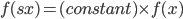
The function retains its form and is scaled according to the scaling factor.

Maxwell's equations are scale invariant.

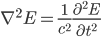
In the absence of currents the charges, the wave equation is

$\nabla^2 E=\frac{1}{c^2} \frac{\partial^2 E}{\partial t^2}$

Using scaling:

$x'=s \times x$
$t'=s \times t\$
$(\nabla^2)' E'=\frac{1}{c^2} \frac{\partial^2 E'}{\partial t'^2}$

$(\nabla^2)'=\frac{1}{s^2}\nabla^2$

$\frac{\partial^2 }{\partial t'^2}=\frac{1}{s^2}\frac{\partial^2 }{\partial t^2}$

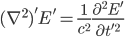
Substituting the value of  scaled variables in the wave equations, it is evident that E' is also a solution.

The entire task of  computational electromagnetism is to solve the wave equation. When we are scaling a quantity, we multiply all the quantities (except frequency )with the scaling factor.Frequency is divided by the scaling factor.
$f=\frac{1}{T}$
$f'=\frac{f}{s}$

Assigning Units¹
Let unit length (eg. nm, cm) be 'a'. Note: in MEEP c=1.

Unit time= (Unit length)/c . Hence unit of time is "a/c" or simply "a".

Frequency =1/(Unit time). Hence frequency is expressed as "c/a" units.

Also note, frequency=c/(wavelength). $f=\frac{1}{\lambda}$

$\omega= 2\pi f, \omega$ is expressed as $2\pi c/a$ units
Optical time period $T=\frac{1}{f}$ (a/c)units

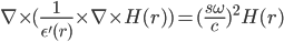
Consider the following equation² :

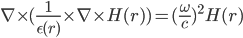$\begin{eqnarray*}\nabla \times (\frac{1}{\epsilon(r)} \times \nabla \times H(r) ) =(\frac{\omega}{c})^2 H(r)\end{eqnarray*}$ --- (1)

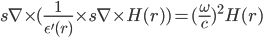
Upon scaling,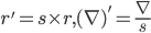$r'=s \times r, (\nabla)'=\frac{\nabla}{s}$
equation (1) becomes
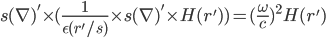$\begin{eqnarray*}s(\nabla)' \times (\frac{1}{\epsilon(r'/s)} \times s(\nabla)' \times H(r') ) =(\frac{\omega}{c})^2 H(r')\end{eqnarray*}$ ---(2)

The following are some useful cases, to extend our analysis from one scale to another.
Case 1: In order to find mode profile of a system where the dielectric constant is either compressed or expanded, i.e 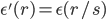$\epsilon '(r)= \epsilon(r/s)$
rewriting the equation:
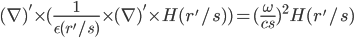$\begin{eqnarray*}(\nabla)' \times (\frac{1}{\epsilon(r'/s)} \times (\nabla)' \times H(r'/s) ) =(\frac{\omega}{cs})^2 H(r'/s)\end{eqnarray*}$ ---(3)

The mode profile in this configuration H'(r')=H(r'/s) is obtained by rescaling the old profile and frequency.

case 2: Analysing a medium in which Dielectric configuration differs everywhere by constant factor of a known profile, i.e, $\epsilon '(r)=\frac{\epsilon(r)}{s^2}$

we can use (1) and substitute $\epsilon '(r)=\frac{\epsilon(r)}{s^2}$. This yields

$\begin{eqnarray*}\nabla \times (\frac{1}{\epsilon '(r)} \times \nabla \times H(r) ) =(\frac{s\omega}{c})^2 H(r)\end{eqnarray*}$ ---(4)

Hence, the same mode profile is obtained by scaling epsilon and frequency. ( $\omega '= s\omega$ )

The equation (4) can also be rewritten in the following form:
$\begin{eqnarray*} s\nabla \times (\frac{1}{\epsilon '(r)} \times s\nabla \times H(r) ) =(\frac{\omega}{c})^2 H(r)\end{eqnarray*}$ ---(5)
The above equation also yields the similar profile by scaling $\epsilon$ and coordinates (r'=sr).

To Summarize:

Step 1: Decide the regime in which you are working, for example micron range and set.

Step 2: Define source parameters : wavelength or frequency.

Step 3: Set the desired run time of the program
Example: 

Consider solving a fiber optic cable with parameters wavelength 1.55µm, Core 8µm diameter and cladding 125µm diameter. Since the domain is in micrometer scale, set a=1µm. Wavelength is 1.55a or simply 1.55. Frequency is 1/1.55. In order to run your simulation for 200 time periods we need to run it for 200/f or 200*1.55 time units. (1 Time period= (1/f)time units)
 

References:

1) MEEP website

2) Photonic Crystals book